The Monetary Policy Cycle
Introduction

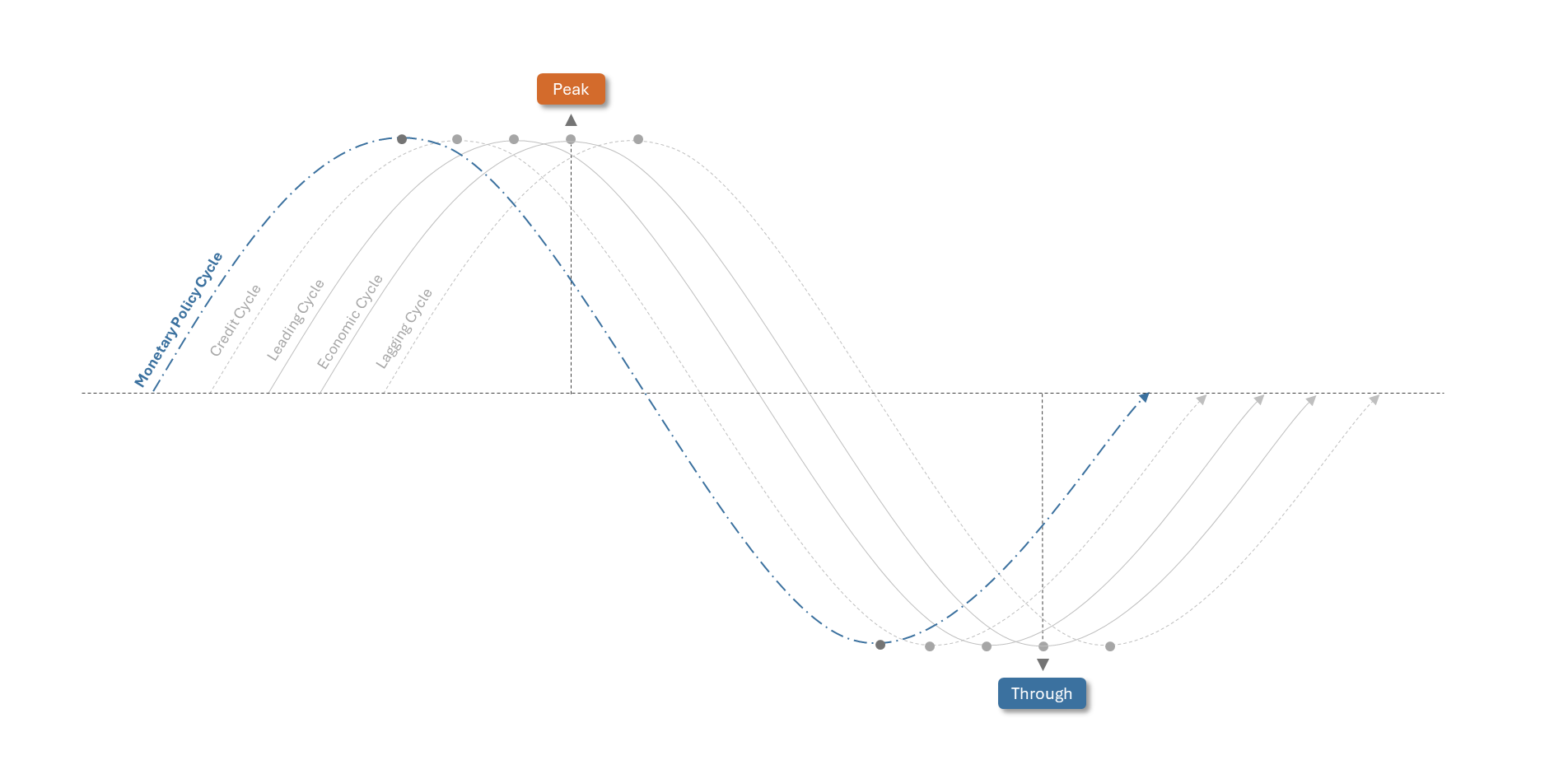
The Monetary Policy Cycle, the first cycle within our cycles within cycles framework
The monetary policy cycle stands as the first and arguably most crucial cycle within our comprehensive “Cycles Within Cycles” framework (Figure 1). It’s the linchpin that sets in motion a series of economic events, ultimately driving the overall business cycle. Through the adjustment of key interest rates and the money supply, central banks like the Federal Reserve exert a powerful influence on economic activity, shaping everything from borrowing costs to investment levels and ultimately, the pace of economic expansion or contraction.
Economic Framework | Cycles Within Cycles
The economy operates in cycles. Our “Cycles Within Cycles” framework helps you understand these cycles—including monetary policy, credit conditions, and leading indicators—to anticipate economic shifts and make informed investment decisions.
Explore the full framework:
Introduction to Cycles Within CyclesThis cycle’s leading nature stems from the proactive stance of central banks. By closely monitoring economic indicators and anticipating future trends, they adjust monetary policy to preemptively address inflationary pressures or stimulate growth. These actions send ripples through the economy, influencing consumer and business behavior, and ultimately dictating the trajectory of the business cycle. Understanding the dynamics of the monetary policy cycle is therefore essential for investors seeking to anticipate market shifts and position their portfolios accordingly.
Defining The Monetary Policy Cycle
Monetary Policy Cycle is the change in policy stance between accommodation and restriction, creatainting a pendulum like effect.
Monetary Policy Cycle
Accomdative
Restrictive
During economic expansions, the yield curve tends to flatten as the Federal Reserve raises short-term interest rates to preempt inflation. This tightening cycle often continues until the yield curve inverts, signaling a potential recession. At the peak of monetary restrictiveness, inflation typically moderates and labor market slack diminishes. As the recession takes hold, the Fed pivots towards aggressive rate cuts to stimulate economic activity, and the cycle begins anew.
The monetary policy cycle can be visualized as a pendulum swinging between accommodation and restriction. This dynamic reflects the Fed’s ongoing efforts to balance economic growth with price stability. The inflection points occur at the extremes of maximum accommodation and maximum restrictiveness, marking turning points in the economic cycle.
The Stages of the Monetary Policy Cycle
The monetary policy cycle unfolds in distinct stages, each characterized by a specific policy stance and economic conditions. These stages reflect the Fed’s evolving response to changing economic dynamics, with the central bank adjusting interest rates and the money supply to achieve its dual mandate of price stability and maximum employment.
The stages of the monetary policy cycle include:
- Restrictive: The initial upward trajectory signals a tightening of monetary policy, aimed at curbing inflation or excessive economic growth.
- Maximum Restrictiveness: The peak of the rate signifies the most stringent monetary stance, where further tightening is unlikely.
- Accommodative: The subsequent decline in the rate marks a shift towards a more supportive monetary policy, intended to stimulate economic activity.
- Maximum Accommodation: The trough of the rate represents the most accommodative policy stance, often seen during periods of economic weakness or towards the end of a recession.
What Influences the Monetary Policy Cycle?
To understand what influences the monetary policy cycle, we need to understand what the objectives of the Federal Reserve are. The Federal Reserve’s dual mandate guides the central bank’s policy decisions.
The Dual Mandate
The Federal Reserve operates under a dual mandate to promote price stability and maximum employment. These objectives guide the Fed’s policy decisions, with the central bank adjusting interest rates and the money supply to achieve these goals. By maintaining stable prices and fostering full employment, the Fed aims to create a conducive environment for sustainable economic growth.
Federal Reserves Report Card The Federal Reserve’s performance in achieving its dual mandate is closely scrutinized by policymakers, economists, and market participants. We hace created a Federal Reserve report Card to evaluate the central bank’s effectiveness in meeting its objectives.
click to veiw the report card:
Driving Monetary Policy is the Federal Reserve’s dual mandate:
- Price Stability: Keeping inflation low and stable
- Maximum Employment: Maximizing employment and minimizing unemployment
Price Stability
Price stability is a cornerstone of the Fed’s mandate, with the central bank targeting an inflation rate of around 2% over the long term. By keeping inflation in check, the Fed aims to preserve the purchasing power of the dollar and prevent runaway price increases that can erode consumer confidence and disrupt economic activity.
Maximum Employment
The Fed also seeks to promote maximum employment, striving to achieve full utilization of the labor market’s resources. By fostering job creation and reducing unemployment, the central bank aims to support economic growth and improve living standards for all Americans.
The Dual Mandate Creates The Fed’s Feedback Loop
A delicate balance between controlling price stability and unemployment
The Federal Reserve’s actions influence the economy through a feedback loop. Where higher unemployment causes lower inflation, and lower inflation causes higher unemployment. Monetary Policy Cycle can be reduced down to the Central Banks balancing act between there dual mandate, with each mandate influencing the other. We classify the both mandates as two sub-cycles to the Monetary Policy Cycle.
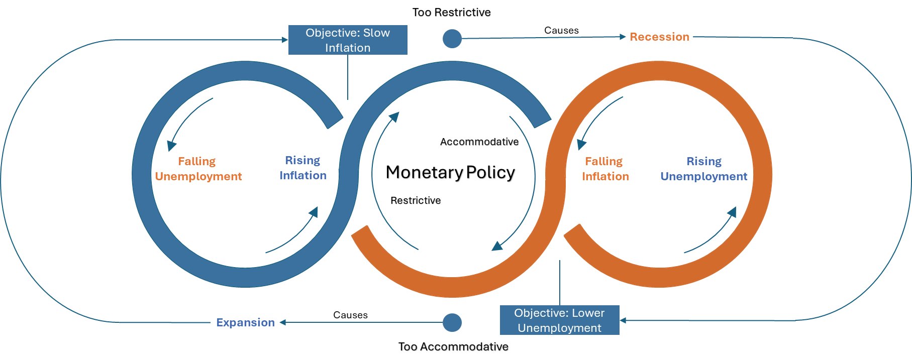
This Feedback Loop identifies two additional sub-cycles
The Labor Cycle
The labor cycle captures the interplay between employment and inflation, with the Fed adjusting policy to promote maximum employment and minimize unemployment. By fostering job creation and reducing unemployment, the central bank aims to support economic growth and improve living standards for all Americans.
The Inflation Cycle
The inflation cycle reflects the relationship between price stability and employment, with the Fed adjusting policy to maintain stable prices and prevent runaway inflation. By targeting an inflation rate of around 2%, the central bank aims to preserve the purchasing power of the dollar and support economic growth.
How The Monetary Policy Drives The Economy
The Federal Reserve (the Fed), as the central bank of the United States, has several powerful tools at its disposal to influence the economy.
Here’s how they can drive expansion or contraction:
- Interest Rates
- Monetary Liquidity
- Forward Guidance
Long and Variable Lags
It is important to note that Monetary policy operates with a lag, meaning it takes time for the full impact of policy changes to be felt in the economy. This lag is what creates the cycles within cycles format that we follow in our modeling.
Interest Rates
The Federal Reserve (the Fed) has a powerful toolkit at its disposal to influence the economy, and interest rate manipulation is a primary weapon in its arsenal. By adjusting key interest rates, the Fed can encourage or discourage borrowing, spending, and investment, thus impacting inflation and overall economic activity. Let’s delve into the specific interest rates under the Fed’s control:
Federal Funds Rate: This is arguably the most well-known and influential rate in the Fed’s toolbox. It’s the target rate that banks charge each other for the overnight lending of reserves. Think of it as the bedrock upon which other interest rates are built. By raising or lowering the federal funds rate target, the Fed sends ripples throughout the financial system, influencing borrowing costs for businesses and consumers alike. This, in turn, affects investment decisions, spending habits, and ultimately, the trajectory of economic growth.
Upper Target: This is the upper end of the Fed’s desired range for the federal funds rate. It acts as a ceiling, preventing the effective federal funds rate from rising too far above the target.
Lower Target: This is the lower end of the Fed’s desired range for the federal funds rate. It acts as a floor, preventing the effective federal funds rate from falling too far below the target.
Effective Federal Funds Rate: the effective fed funds rate is the actual, realized rate that prevails in the market. It’s calculated as a weighted average of all the overnight interbank lending transactions that occur each day. While heavily influenced by the Fed’s target, the effective rate can fluctuate slightly based on market dynamics, such as the supply and demand for reserves, liquidity conditions, and bank behavior.
Discount Rate: This is the rate at which commercial banks can borrow money directly from the Fed, acting as a lender of last resort. It’s typically maintained above the federal funds rate to encourage banks to exhaust other borrowing options first. By adjusting the discount rate, the Fed can influence the overall cost of credit in the system and provide a safety net for banks facing liquidity challenges. This rate plays a crucial role in maintaining financial stability and ensuring the smooth functioning of the banking system.
Repo Rate (Repurchase Agreement Rate): This is the interest rate at which the Fed lends money to eligible counter parties (like money market funds) in exchange for U.S. Treasury securities as collateral. It’s a critical tool for managing short-term interest rates and ensuring liquidity in the financial system. By adjusting the repo rate, the Fed can fine-tune the supply of reserves in the banking system, influencing the overall level of interest rates and impacting borrowing costs for a wide range of financial institutions.
Interest on Reserves: This is the interest rate paid by the Fed to banks on the reserves they hold at the central bank. It acts as a floor for short-term interest rates and incentivizes banks to maintain certain reserve levels. By adjusting this rate, the Fed can influence the amount of reserves held by banks, impacting the overall supply of money in the system and affecting lending activity. This tool provides another lever for the Fed to manage monetary conditions and guide the economy toward its goals.
| Apr 11 | Apr 04 | Mar 28 | Mar 21 | Mar 14 | Mar 07 | Feb 28 | Feb 21 | Feb 14 | Feb 07 | Jan 31 | Jan 24 | |
|---|---|---|---|---|---|---|---|---|---|---|---|---|
| Upper Target | 4.50 | 4.50 | 4.50 | 4.50 | 4.50 | 4.50 | 4.50 | 4.50 | 4.50 | 4.50 | 4.50 | 4.50 |
| Discount Rate | 4.33 | 4.33 | 4.33 | 4.33 | 4.33 | 4.33 | 4.33 | 4.33 | 4.33 | 4.33 | 4.33 | 4.33 |
| Effective Federal Funds Rate | 4.33 | 4.33 | 4.33 | 4.33 | 4.33 | 4.33 | 4.33 | 4.33 | 4.33 | 4.33 | 4.33 | 4.33 |
| Interest On Reserve balances | 4.40 | 4.40 | 4.40 | 4.40 | 4.40 | 4.40 | 4.40 | 4.40 | 4.40 | 4.40 | 4.40 | 4.40 |
| Federal Funds Target Rate | 4.33 | 4.33 | 4.33 | 4.33 | 4.33 | 4.33 | 4.33 | 4.33 | 4.33 | 4.33 | 4.33 | 4.33 |
| Overnight Reverse Repurchase | 4.25 | 4.25 | 4.25 | 4.25 | 4.25 | 4.25 | 4.25 | 4.25 | 4.25 | 4.25 | 4.25 | 4.25 |
| Lower Target | 4.25 | 4.25 | 4.25 | 4.25 | 4.25 | 4.25 | 4.25 | 4.25 | 4.25 | 4.25 | 4.25 | 4.25 |
Monitor Interest Rate Perceptions in the Market
Monetary Policy Risk (The Risk of Δ in the Risk Free Rate)
The risk-free rate, representing the theoretical return achievable without risk, forms the bedrock of asset pricing and the foundation upon which risk premiums are built. Investors demand compensation, in the form of higher returns, for assuming incremental risk relative to this baseline.
Federal Reserve policy plays a pivotal role in shaping market risk premiums by directly influencing the risk-free rate. Through adjustments to the federal funds rate, and the subsequent impact on short-term interest rates, the central bank exerts significant influence over the expected returns of diverse asset classes and investment strategies.
The risk-free rate is intrinsically linked to the monetary policy cycle. The Federal Reserve’s setting of the target range for the federal funds rate propagates through the economy, affecting short-term interest rates and broader liquidity conditions. These cyclical shifts impact various asset classes and investment strategies differential, with sector- and security-specific sensitivities to interest rate and liquidity changes.
In our modeling, we term this influence “monetary policy risk,” which is effectively captured by the prevailing risk-free rate. Specifically, for our machine learning applications, we utilize the 1-Month Treasury Bill Secondary Market Rate as a proxy for this risk-free rate.
| Apr 11 | Apr 04 | Mar 28 | Mar 21 | Mar 14 | Mar 07 | Feb 28 | Feb 21 | Feb 14 | Feb 07 | Jan 31 | Jan 24 | |
|---|---|---|---|---|---|---|---|---|---|---|---|---|
| One Month Treasury Yields | -- | 4.36 | 4.38 | 4.36 | 4.37 | 4.38 | 4.38 | 4.36 | 4.37 | 4.37 | 4.37 | 4.45 |
| Δ in One Month Treasury Yields | -- | -0.02 | 0.02 | -0.01 | -0.01 | 0.00 | 0.02 | -0.01 | 0.00 | 0.00 | -0.08 | 0.02 |
Near-Term Spreads
There are two primary near term spreads that we monitor:
- Near-term forward spread (NTFS): a measure of the expected change in short-term interest rates over the next 18 months. It is calculated as the difference between the expected 3-month interest rate 18 months from now and the current 3-month yield.
- Near-term spread (NTS): The yield curve spread between the 2-year and 3-month Treasury yields. This is a closely watched measure in the fixed income market and provides valuable insights into market expectations and potential economic trends.
The NTFS & NTS are good indicators of the future stance of monetary policy as well as recessions. When the spreads are positive, it suggests that the market expects the central bank to tighten monetary policy in the near future. This can be a sign that the economy is strong and that inflation is a concern. Conversely, when the spreads are negative, it suggests that the market expects the central bank to loosen monetary policy. This can be a sign that the economy is weakening and that a recession is possible.
The NTFS is a relatively new indicator, but it has been shown to be a reliable predictor of recessions.
In a 2019 paper, Engstrom and Sharpe found that the NTFS had a better track record of predicting recessions than the traditional yield curve spread between 10-year and 2-year Treasury yields.
| Apr 11 | Apr 04 | Mar 28 | Mar 21 | Mar 14 | Mar 07 | Feb 28 | Feb 21 | Feb 14 | Feb 07 | Jan 31 | Jan 24 | |
|---|---|---|---|---|---|---|---|---|---|---|---|---|
| Near-Term Forward Spread (NTFS) | -- | -- | -0.45 | -0.41 | -0.31 | -0.32 | -0.36 | -0.10 | 0.01 | 0.01 | 0.00 | 0.09 |
| Δ NTFS | -- | -- | -0.04 | -0.10 | 0.01 | 0.03 | -0.26 | -0.11 | 0.00 | 0.02 | -0.09 | 0.00 |
| Near-Term Spread (NTS) | -- | -0.6 | -0.44 | -0.39 | -0.31 | -0.35 | -0.33 | -0.13 | -0.08 | -0.06 | -0.09 | -0.08 |
| Δ NTS | -- | -0.16 | -0.05 | -0.08 | 0.04 | -0.02 | -0.20 | -0.05 | -0.02 | 0.03 | -0.01 | -0.01 |
Warning: Neat-Term Forward Spread is Inverted
The Near-Term Spread is at -0.45. When the near-term forward spread is inverted, it typically signals that investors expect short-term interest rates to decrease in the near future. This could indicate a perceived slowdown in economic activity or the anticipation of the Federal Reserve cutting rates to stimulate the economy.
Warning: Neat-Term Spread is Inverted
The Near-Term Spread is at -0.6. When the near-term spread is inverted, it typically signals that investors expect short-term interest rates to decrease in the near future. This could indicate a perceived slowdown in economic activity (including a recession) or the anticipation of the Federal Reserve cutting rates to stimulate the economy.
Monetary Liquidity Injections
Monetary liquidity injections refer to actions undertaken by a central bank, like the Federal Reserve, to increase the supply of money within the financial system.
Formula for Liquidity Injections from the Federal Reserve
\[ Liquidity = Assets - TGA - RRP - OL \] Where:
- Liquidity is the Fed Liquidity being injected into the economy.
- Assets is the total assets on the Federal Reserve balance sheet.
- TGA is the Treasury General Account.
- RRP is the reverse repurchase agreements.
- OL is the operating losses realized by the Federal Reserve.
Let’s break down each component:
Assets: This represents the total assets held by the Federal Reserve, primarily consisting of U.S. Treasury securities and agency mortgage-backed securities. When the Fed purchases these assets through open market operations, it injects liquidity into the system.
TGA (Treasury General Account): This is the U.S. Treasury’s checking account at the Federal Reserve. Increases in the TGA balance effectively drain liquidity from the system, as funds are moved from the economy to the Treasury’s account.
RRP (Reverse Repurchase Agreements): These are transactions where the Fed temporarily drains liquidity by selling securities to eligible counterparties with an agreement to repurchase them later. This helps set a floor under short-term interest rates.
OL (Operating Losses): While less frequent, the Fed can realize operating losses, for example, if interest rates rise and the return on its asset holdings falls below the interest it pays on reserves. These losses reduce the Fed’s capital and, in turn, decrease the overall liquidity in the system.
By monitoring the changes in these components, we can gauge the net impact of the Fed’s actions on liquidity conditions. Increases in liquidity tend to ease financial conditions, potentially leading to lower interest rates and increased economic activity. Conversely, decreases in liquidity tighten financial conditions, potentially raising interest rates and slowing economic growth.
Interpritation of Feds Liquidity Creation Components
- A Decrease movement in any of the liquidity components represent liquidity being added into the financial system.
- A Increase movement suggests that liquidity is being removed from the economy.
A high RRP market represents excess liquidity in the market.
Interpritation
We summed the components of liquidity creation and inverted the resulting chart. This allows us to visualize money leaving the financial system and entering the private sector as an upward trend, indicating increased liquidity.
Liquidity Creation Components
| Apr 11 | Apr 04 | Mar 28 | Mar 21 | Mar 14 | Mar 07 | Feb 28 | Feb 21 | Feb 14 | Feb 07 | Jan 31 | Jan 24 | |
|---|---|---|---|---|---|---|---|---|---|---|---|---|
| Δ Treasury General Account (Millions) | -- | -14346 | -99,829.00 | -34,914.00 | -72,105.00 | -45,732.0 | -170,388.00 | -70,216.00 | -8,799.00 | 6,404.00 | 146,064.0 | 14,298.00 |
| Δ Reverse Repo Market (Millions) | -- | -102076 | 85,725.00 | 74,616.00 | -10,071.00 | -98,117.0 | 165,439.00 | 10,213.00 | -36,478.00 | -92,665.00 | 82,941.0 | -13,355.00 |
| Δ Fed Operating Losses (Millions) | -- | -746 | -985.00 | -526.00 | -116.00 | 224.0 | -920.00 | -499.00 | -1,811.00 | 379.00 | -1,471.0 | -1,114.00 |
| Δ Fed Liquidity (Millions) | -- | -- | -27,271.71 | -28,869.57 | 72,296.43 | 145,643.7 | -45,521.43 | 61,094.71 | 54,321.14 | 85,915.29 | -201,812.0 | -45,334.71 |
| Δ Total Liquidity Components (Millions) | -- | -- | 9,403.00 | 20,497.71 | -71,783.14 | -151,257.3 | 30,073.86 | -89,242.86 | -64,260.86 | -90,851.43 | 188,159.7 | 37,374.43 |
Federal Reserve’s Liquidity Injections
| Apr 11 | Apr 04 | Mar 28 | Mar 21 | Mar 14 | Mar 07 | Feb 28 | Feb 21 | Feb 14 | Feb 07 | Jan 31 | Jan 24 | |
|---|---|---|---|---|---|---|---|---|---|---|---|---|
| Δ Total Liquidity Components (Millions) | -- | -- | 9,403.00 | 20,497.71 | -71,783.14 | -151,257.3 | 30,073.86 | -89,242.86 | -64,260.86 | -90,851.43 | 188,159.7 | 37,374.43 |
| Δ Federal Reserve Balance Sheet (Millions) | -- | -16801 | -15,729.00 | -3,589.00 | 2,807.00 | -9,337.0 | -16,231.00 | -31,181.00 | 2,578.00 | -7,251.00 | -13,574.0 | -2,310.00 |
| Δ Fed Operating Losses (Millions) | -- | -746 | -985.00 | -526.00 | -116.00 | 224.0 | -920.00 | -499.00 | -1,811.00 | 379.00 | -1,471.0 | -1,114.00 |
| Δ Fed Liquidity (Millions) | -- | -- | -27,271.71 | -28,869.57 | 72,296.43 | 145,643.7 | -45,521.43 | 61,094.71 | 54,321.14 | 85,915.29 | -201,812.0 | -45,334.71 |
Fed Liquidity is increasing.
This is usually positive for equity markets as aditional liquidity usually flows into the equity markets.
The Impact of the Monetary Policy Cycle
We measure the impact of the Monetary Policy Cycle on three levels:
- Impact on the business Cycle
- Impact on Risk Factors
- Impact on Financial Markets
Impact on the Business Cycle
The monetary policy cycle plays a critical role in shaping the stages of the business cycle, influencing economic activity and market dynamics throughout the cycle’s phases. By adjusting interest rates and the money supply, the Fed can stimulate or restrain economic growth, setting the stage for the following stages of the business cycle.
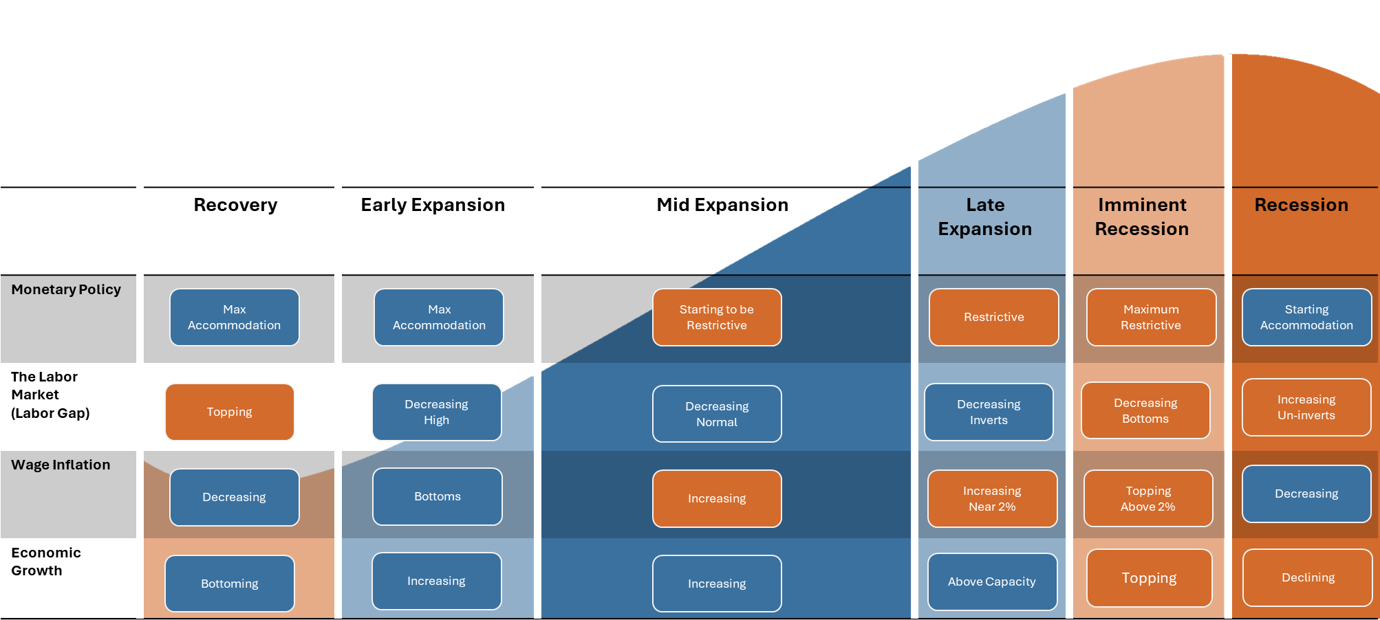
Recovery
During the recovery phase, the Fed typically maintains an accommodative policy stance, with low-interest rates and ample liquidity supporting economic growth. By providing stimulus to the economy, the central bank aims to foster a robust recovery and set the stage for sustained expansion.
Early Expansion
As the economy enters the early expansion phase, the Fed may begin to tighten monetary policy, raising interest rates to prevent inflationary pressures from building. By gradually withdrawing stimulus, the central bank aims to maintain price stability and prevent overheating in the economy.
Mid Expansion
In the mid-expansion phase, the Fed continues to tighten policy, gradually raising interest rates to moderate economic growth and prevent imbalances from emerging. By adjusting monetary policy in a measured manner, the central bank aims to sustain the expansion while avoiding excessive inflation.
Late Expansion
During the late expansion phase, the Fed may adopt a more aggressive tightening stance, raising interest rates to cool off an overheating economy. By tightening policy, the central bank aims to prevent inflation from spiraling out of control and maintain economic stability.
Imminent Recession
As the economy approaches a recession, the Fed pivots towards an accommodative policy stance, cutting interest rates to stimulate economic activity and support financial markets. By providing liquidity to the economy, the central bank aims to cushion the impact of the downturn and lay the groundwork for recovery.
Recession
During a recession, the Fed typically adopts an aggressive easing stance, lowering interest rates and implementing unconventional policy measures to support the economy. By providing stimulus to the economy, the central bank aims to jumpstart growth and restore confidence in financial markets.
Rise in Unemployment is a Recession
The relationship between real GDP growth and changes in the unemployment rate is inverse. As economic growth increases, unemployment tends to fall. Conversely, during recessions, unemployment rises as economic activity contracts. Okuns law shows us that a recession occurs when unemployment rises, and GDP growth falls.
This relationship can be viewed through the following regression chart:
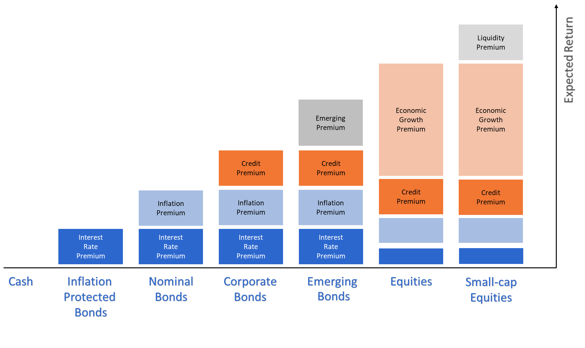
Impact on Macroeconomic Factors
Understanding how risk is accounted for in asset pricing is essential for investors. A key concept in this relationship is the risk premium, which represents the additional return investors demand for bearing risk beyond that of a risk-free investment. The risk premium varies across asset classes, with riskier assets offering higher expected returns to compensate for the additional risks they carry.
In Figure 20, we illustrate how different asset classes offer varying levels of expected return based on the risks they carry. From the safety of cash to the higher growth potential of equities, each investment comes with its own set of risk premiums. The risk free rate is the foundation of risk premiums, with investors demanding higher returns for taking on additional risks.
Impact on Financial Assets & Investment Play Book
Monetary Policy Cycle can impact various asset classes and investment strategies, with different sectors and securities responding differently to changes in interest rates and liquidity conditions.
While it impacts many asset classes, we are focusing on the impact that can be isolated to the Monetary Policy Cycle, Mainly short-duration treasuries.
| Total Sample | Max Restrictive | Accomdative | Max Accodative | Restrictive | |
|---|---|---|---|---|---|
| Short-Term Treasury ETF (SHV) | 1.43 | 4.68 | 3.42 | 0.03 | 1.46 |
| TIPS ETF (TIP) | 3.56 | 4.97 | 0.46 | 7.74 | 1.32 |
| 1-3 Year Treasury Bond ETF (SHY) | 1.93 | 5.59 | 0.41 | 0.70 | 5.83 |
| MBS ETF (MBB) | 2.56 | 7.08 | 5.22 | 2.32 | -0.64 |
| 3-7 Year Treasury Bond ETF (IEI) | 2.91 | 7.69 | 10.12 | 1.51 | -0.58 |
| 7-10 Year Treasury Bond ETF (IEF) | 3.70 | 12.72 | 1.98 | -0.44 | 9.02 |
| 10-20 Year Treasury Bond ETF (TLH) | 3.15 | 8.93 | 13.10 | 2.32 | -3.34 |
| 20+ Year Treasury Bond ETF (TLT) | 4.04 | 19.30 | 0.97 | -1.23 | 10.37 |
Total Sample Max Restrictive Accomdative
Short-Term Treasury ETF (SHV) 1.43 4.68 3.42
TIPS ETF (TIP) 3.56 4.97 0.46
1-3 Year Treasury Bond ETF (SHY) 1.93 5.59 0.41
MBS ETF (MBB) 2.56 7.08 5.22
3-7 Year Treasury Bond ETF (IEI) 2.91 7.69 10.12
7-10 Year Treasury Bond ETF (IEF) 3.70 12.72 1.98
10-20 Year Treasury Bond ETF (TLH) 3.15 8.93 13.10
20+ Year Treasury Bond ETF (TLT) 4.04 19.30 0.97
Max Accodative Restrictive
Short-Term Treasury ETF (SHV) 0.03 1.46
TIPS ETF (TIP) 7.74 1.32
1-3 Year Treasury Bond ETF (SHY) 0.70 5.83
MBS ETF (MBB) 2.32 -0.64
3-7 Year Treasury Bond ETF (IEI) 1.51 -0.58
7-10 Year Treasury Bond ETF (IEF) -0.44 9.02
10-20 Year Treasury Bond ETF (TLH) 2.32 -3.34
20+ Year Treasury Bond ETF (TLT) -1.23 10.37
Investment Play Book
Government Bond Management Playbook Based on Monetary Policy Cycle
Objective: Optimize government bond portfolio returns while minimizing risk through active management aligned with the monetary policy cycle.
Investment Philosophy:
- Loss Avoidance: Prioritize capital preservation, especially during restrictive monetary policy phases.
- Cycle Awareness: Actively monitor and anticipate shifts in the monetary policy cycle.
- Adaptive Management: Dynamically adjust bond portfolio duration and allocations based on the prevailing and anticipated monetary policy stance.
Monetary Policy Cycle Phases and Corresponding Strategies:
- Maximum Accommodative:
Characteristics: Central banks pause on rate cuts, reaching the lower bound on inters rates.
Bond Strategy:
- Reduce duration: Focus on short-term bonds (e.g., TFLO, SHV) to minimize interest rate risk.
- Consider TIPS: If inflation expectations are rising, allocate a portion to TIPS (TIP) as a hedge.
- Seek higher yield: Explore opportunities in higher-yielding sectors (e.g., corporate bonds) while maintaining a cautious approach.
- Accommodative:
Characteristics: Central bank maintaining an accommodative stance; interest rates remain low; continued liquidity support.
Bond Strategy:
- Gradually increase duration: Shift towards slightly longer-duration bonds (e.g., SHY) as yields begin to rise.
- Maintain TIPS exposure: Continue to hold TIPS as an inflation hedge.
- Monitor credit spreads: Actively assess credit risk and adjust corporate bond exposure accordingly.
- Restrictive:
Characteristics: Central bank shifting to a restrictive stance; interest rates rising; liquidity tightening.
Bond Strategy:
- Shorten duration: Reduce exposure to longer-term bonds (e.g., IEI, IEF, TLH, TLT) to mitigate interest rate risk.
- Reduce TIPS exposure: As inflation expectations moderate, reduce TIPS allocation.
- Focus on quality: Favor high-quality government bonds to minimize credit risk.
- Maximum Restrictive:
Characteristics: Central bank aggressively tightening policy; interest rates peaking; liquidity significantly reduced.
Bond Strategy:
- Maintain short duration: Hold primarily short-term bonds (e.g., TFLO, SHV) to preserve capital.
- Consider opportunistic increases in duration: Selectively add longer-term bonds (e.g., IEF, TLT) during market downturns to enhance yield potential.
Risk Management:
Stay vigilant: Closely monitor economic data and central bank communications for signs of a policy shift. Key Considerations:
Yield Curve: Actively analyze the yield curve shape to identify opportunities and risks. Credit Spreads: Monitor credit spreads to assess the risk-reward profile of corporate bonds. Inflation Expectations: Incorporate inflation expectations into bond allocation decisions. Economic Outlook: Continuously assess the overall economic outlook and its potential impact on the monetary policy cycle. Disclaimer: This playbook provides general guidance for managing government bonds during different monetary policy cycle phases. Specific investment decisions should be made based on individual circumstances and risk tolerance.